هو الشخص الذى يقوم بعمل الشى باعلى جودة واقل تكلفة
لذلك التكلفة الاقتصادية من اهم مايتعرض له المهندس فى العمل فعليه ان تكون فى اعتباره اولا
هناك فرق كبير بين مادة الاقتصاد الهندى ومادة الاقتصاد العادية
وهى اننا فى كلية الهندسة الناتج يكون له مدلول تطبيقى وعملى فى الحياة العملية على عكس الطالب بكلية تجارة او غيرها من الكليات النظرية فالناتج يمثل بالنسبة له رقم لايهم ان كان سالبا او موجبا .....إلخ
لماذا المهندسين بحاجة إلى أن تعلم علم الاقتصاد؟
منذ زمن بعيد، وكانت الحواجز الأكثر أهمية للمهندسين هى الحواجز التكنولوجية. الأشياء التي المهندسينيريدوا ان يفعلوها، انهم ببساطة لا يعرفون حتى الآن كيفية القيام بذلك، أو لم تضع حتى الآن الأدوات اللازمة لذلك. هناك بالتأكيد العديد من التحديات أكثر مثل هذه التي تواجه في الوقت الحاضر المهندسين. ومع ذلك، فقد وصلنا إلى نقطة في الهندسة حيث لم يعد من الممكن، في معظم الحالات، وذلك ببساطة لتصميم وبناء الأشياء من أجل ببساطة من تصميم وبناء عليها. الموارد الطبيعية (من الذي يجب أن نبني الأشياء) أصبحت أكثر نادرة وباهظة الثمن أكثر من ذلك. نحن أكثر وعيا من الآثار الجانبية السلبية من الابتكارات الهندسية (مثل تلوث الهواء الناجم عن السيارات) من أي وقت مضى.
لهذه الأسباب، وكلف المهندسين أكثر وأكثر لوضع أفكار المشاريع الخاصة بهم ضمن الإطار الأوسع للبيئة في كوكب معين، والبلد، أو المنطقة. يجب أن يسألوا أنفسهم إذا المهندسين مشروع معين سوف نقدم بعض الفائدة الصافية للناس الذين سيتأثرون بالمشروع، وبعد النظر في الفوائد الكامنة، بالإضافة إلى أي آثار جانبية سلبية (العوامل الخارجية)، بالإضافة إلى تكلفة استهلاك الموارد الطبيعية، على حد سواء في الثمن الذي يجب أن تدفع لهم، وإدراك أن مرة واحدة يتم استخدامها لهذا المشروع، وسوف لن تكون متاحة للأي مشروع آخر

Engineering economics
يعرف الاقتصاد الهندسى على انه جعل مادة الاقتصاد تخدم التطبيقات فى المشوعات الهندسية حيث يبحث المهندسون دائما على حلول اقتصادية لجعل مشروعاتهم اوسثمارتهم اكثر عائدا وربحا
حيث الاقتصاد الهندسى يعرف ايضا على انه مجموعة من الطرق الاقتصادية التى تستخدم التحليل المنطقى للبدائل حتى يتم اتخاذ القرار المناسب للحصول على اعلى جودة باقل تكلفة
وعليه فأن علم الاقتصاد يختص بدراسة الموضوعات التالية
أولا:- تخصيص الموارد
ثانيا :- تنظيم الإنتاج
ثالثا :- توزيع الإنتاج
رابعا :- كفاءة استخدام الموارد
أولا تخصيص الموارد
============
المورد الاقتصادي متجدد وغير متجدد .
المورد الاقتصادي النادر .
استهلاكنا منه يؤثر في استهلاك الآخرين منه .
المورد الاقتصادي دائما له سعر و ثمن .
الموارد البشرية :- وهي تعتبر من أهم الموارد الاقتصادية و عادة ما يقوم الاقتصاديون بوضعها على رأس الموارد و ذالك لأهمية دورها في النمو و تقدم أي نظام .
فالمورد البشري في رأي الاقتصاديون مفضل على بقية الموارد الأخرى المتوفرة لاقتصادها و يستدل على أهمية المورد البشري في التنمية الاقتصادية إلى ما وصلت إليه اليابان من تقدم مع أنها تفتقر إلى أغلب الموارد الأولية اللازمة لنهضة صناعتها , فبرغم من عدم توفر النفط و الفحم و الحديد إلا أنها اعتمدت على الموارد البشرية المتطورة التي استطاعت إن تنافس اكتر البلدان تقدما صناعيا
الموارد الطبيعية :- ويطلق على هذا النوع من الموارد اسم الموارد الأرضية و يمكن حصرها في كل ما يوجد على سطح الأرض من زراعة و أنهار و غابات و كذالك ما يوجد في باطنها من مياه جوفية و نفط و غير ذالك .
رأس المال :- يشمل هذا النوع من الموارد كل الإنشاءات من الطرق والكباري والمصانع و الآلات , فكلما زاد هذا المورد في بلد ما كانت فرص التنمية الاقتصادية بها اكتر يسرا من تلك البلاد التي تفتقر إلى هذا النوع من الموارد .
التنظيم و الإدارة :- هدا المورد له صلة وثيقة بالمورد البشري حيت المنظم هو المسئول عن دفع عوامل الإنتاج في الوحدة الإنتاجية بنسب محددة كفيلة بإعطاء كفاءة عالية في الإنتاج و يتوقف على المنظم بالدرجة الأولى مدى إمكانية إدخال التكنولوجيا الحديثة و الاختراعات و تطويعها للعملية الإنتاجية للحصول على اكبر قدر ممكن من الإنتاج بنفس الكمية من عوامل الإنتاج .
ثالثا :- توزيع الإنتاج
================
رابعا :- كفاءة استخدام الموارد
==============
ـــــــــــــــــــــــــــــــــــــــــــــــــــــــــــــــــــــــــــــــــــــــــــــــــــــــــــــــــــــــــــــــــــــ
الجدوى الاقتصادية للمشاريع الهندسية
المراحل الزمنية اللازمة لتحقيق المشروع :-
هناك مراحل و خطوات إدارية و قانونية و فنية متعددة يمر بها كل مشروع فالدراسة الفنية للمشروع تقتضي أعداد جدول زمني مبسط يبين متوسط المدة اللازمة لكل مرحلة مقدرة بعدد الأشهر يتم بعد دالك وضع مخطط يوضح المراحل الزمنية المختلفة اللازمة لتحقيق المشروع حسب تعاقبها الزمني و لا تعد هذه المراحل ثابتة لكل مشروع حيت يمكن دمج هذه المراحل مع بعضها البعض أو أن تضاف إليها مراحل جديدة و ذالك حسب احتياجات كل مشروع و مدى تقيد الجهات الأخرى بالتزاماتها حول المشروع و بالتالي يمكن تصنيف المراحل الزمنية لتحقيق المشروع إلى فئتين أساسيتين :-
الفئة الأولى :- تشمل المراحل الزمنية التي يمر بها المشروع قبل توقيع العقد و تسمى هذه المراحل بالمراحل الإدارية .
الفئة الثانية :- تشمل المراحل الزمنية التي يمر بها المشروع بعد توقيع العقد و تسمى هذه المراحل بالمراحل التنفيذية.
دراسة الجدوى الاقتصادية للمشروع :-
أن اتخاذ القرار بإقامة أي مشروع اقتصادي يعني بالضرورة تخصيص جزء من الموارد في سبيل الحصول على المنافع المرتقبة منه , وهذا يعني أعطاء دالك المشروع الأفضلية على مشروعات أخرى مقترحة أو يمكن اقتراحها لا من ناحية استخدامه الموارد المتاحة فحسب و أنما من ناحية منافعه الاقتصادية بالنسبة إلى غيره من المشروعات الاقتصادية لذا تجب المفاضلة بين مختلف المشروعات المقترحة لمعيار محدد قبل تبني أي منها واختياره للتنفيذ .
يعطي الجدول التالي فكرة عن أهم المراحل الزمنية التي يمر بها اغلب المشروعات

==========
الإنفاق في المشاريع
===========
الإنفاق الذي يتطلبه المشروع بعد بدءه بالإنتاج من نفقات مختلفة .
الإنفاق الذي ستلزمه تشغيل المشروع سنة بعد سنة طوال العمر المقدر له و يسمى تكاليف التشغيل أما الموارد الذي يحققه المشروع المقترح فهي موارد سوف يحصل عليها مقابل بيع منتجاته أو مقابل خدمات يقدمها للغير خلال العمر المقدر له .
تعريف دراسة الجدوى الاقتصادية :- تعرف دراسة الجدوى بأنها مجموعة من الأسس العلمية المستمدة من علم الاقتصاد و الإدارة و بحوت العمليات و التي تستخدم في تجميع البيانات و دراستها و تحليلها بهدف تقييم المشروعات الاستثمارية أو تحديد صلاحيتها من عدة جوانب قانونيا و تسويقيا وفنيا و ماليا و اجتماعيا عليه فأن دراسة الجدوى هي أسلوب علمي لتقدير احتمالات نجاح أو فشل مشروع معين أو فكرة استثمارية أو قرار استثماري قبل التنفيذ الفعلي و ذالك في ضوء قدرة المشروع أو القرار الاستثماري على تحقيق أهداف معينة للمستثمر و للمجتمع ككل .
تحديد هدف الدراسة
الدراسة التمهيدية للجدوى
الدراسة التفصيلية للمشروع
تقييم المشروع
تنفيذ المشروع
الدراسة التمهيدية للجدوى :- تهدف الدراسة إلى تحديد دقيق و تفصيلي للوضع الاقتصادي العام للدولة المعنية و أهمية القطاع الذي ينتمي إليه المشروع , وأهم العناصر الذي تشتمل عليها دراسة الوضع الاقتصادي العام للدولة
1. حجم السكان في الدولة المعنية و معدل النمو و متوسط دخل الفرد .
2. قوة العمل و توزيعه الجغرافي و القطاعي .
3. الموارد الطبيعية و الاحتياط المتاح .
4. الناتج المحلي و الإجمالي و توزيعاتها القطاعية
5. تراكم الديون الخارجية و أعباء خدمة الدين .
6. بيان أهمية القطاع الصناعي في الهيكل التركيبي الاقتصادي الوطني
7. بيان المشروعات المنفذة و التي هي قيد التنفيذ ذات العلاقة بأهداف المشروع
في الواقع تحرص الدراسة التمهيدية في تقريرها على إعطاء إجابات واضحة على التساؤلات التالية
1. ما مدى احتمال لنجاح المشروع على القيام بالدراسة التفصيلية ؟
2. ما هي الجوانب التي تحتاج إلى مزيد من الجهد عند إعداد الدراسة التفصيلية ؟
3. ما التكلفة المتوقعة للدراسة التفصيلية ؟
الدراسة التفصيلية للمشروع :- تبدأ بعمل دراسة للجدوى القانونية و البيئية و دراسة الجدوى التسويقية و دراسة الجدوى الفنية و الهندسية ثم دراسة الجدوى المالية و التجارية و أخيرا دراسة الجدوى الاجتماعية .
إذا كانت هذه الدراسات ايجابية يتم وضع قيمة لدرجة ايجابية هذه الفرصة الاستثمارية باستخدام احد المعايير المتعارف عليها لتقييم إجراءات الإنشاء و التأسيس و تشمل الدراسة التفصيلية ما يلي :-
دراسة قانونية .
دراسة تسويقية .
دراسة فنية و هندسية وتشمل الأتي :-
تقييم المشروع .
اتخاذ القرار .
الإنشاء و التأسيس .
تجارب التشغيل .
التشغيل الفعلي .
دراسة مالية .
دراسة اجتماعية .
دراسة الجدوى التسويقية
- دراسة السوق :- هي عملية جمع و فرز و تحليل المعلومات المتعلقة بالمنتجات والأسواق والزبائن والشركات المنافسة و العمليات التجارية المختلفة .
تستخدم دراسة السوق عندما ترى الشركة أن هناك فرصة أمامها بالسوق المحلية أو الخارجية مما يجعلها بحاجة إلى بناء قاعدة معرفية صلبة تبني عليها قراراتها الإستراتيجية ويمكن استخدام دراسة السوق للأغراض التالية
التعرف على الاحتياجات الحالية للسوق .
تقييم مدى الحاجة إلى منتجات جديدة .
تحديد سياسة التسويق و التسعير .
اختيار مواقع المعامل و المستودعات .
القيام بعمليات التوسع .
تقديم التأييد و الدعم للأفكار الجديدة .
في الدول النامية لا تأخذ دراسة الجدوى التسويقية في عين الاعتبار للأسباب التالية
الاعتقاد السائد بين المخططين في هذه الدول أن المشاكل الأساسية التي تواجه عمليات التنمية تتمثل في المشاكل الإنتاجية و التمويلية و ليس مشاكل التسويق و سبب دالك يعود إلى مستويات التنمية .
عدم وجود استقرار سياسي مما يؤدي إلى ركود اقتصادي و كساد حركة السوق .
عدم توافر الخبرات التسويقية اللازمة لأجراء مثل هده الدراسة .
عدم توافر البيانات و المعلومات اللازمة لأجراء مثل هده الدراسة .
عدم توافر الأدوات و الأجهزة المساعدة التي تتطلبها الدراسة التسويقية
ضعف الوعي التسويقي وإهمال رغبة المستهلك .
يمكن تعريف الدراسة الفنية و الهندسية للمشاريع الهندسية بأنها تلك الدراسة المتعلقة بتحديد مدى قابلية المشروع موضع الدراسة للتنفيذ من عدمه .
بالإضافة إلى الحصول على المعلومات الخاصة بكل من الإنفاق الرأسمالي (تكلفة الأرض – المباني – المعدات ) و الإنفاق الجاري كما تؤدي عدم الدقة في أعداد الدراسات الفنية و الهندسية إلى الوصول إلى تقديرات غير سليمة للتكاليف الرأسمالية و التجارية مما يؤدي إلى سوء تقدير حجم الاستثمار و بالتالي إلى احتمال وقوع المشروع في مشاكل مالية سواء أكانت في التمويل أو السيولة , و يقوم بأجراء هذه الدراسة الفنيون و الخبراء الدين تمكنهم تخصصاتهم من الحكم على صلاحية مختلف الجوانب الفنية اللازمة لإنشاء المشروع.
تشمل الدراسة الفنية عدة مواضيع متشعبة ليتمكن القائم بدراسة الجدوى من إعداد تصور نهائي للنتائج التي يمكن عن طريقها الحكم على مدى توافر عوامل نجاح المشروع .
مدى توفر الخامات و الأيدي العاملة و الخدمات المختلفة
مدى تشتت الطلب أو تركيزه على منتجات المشروع
الحجم الاقتصادي للعمليات الإنتاجية
وذالك لما يترتب عليه من نتائج يمتد تأثيرها لفترة طويلة من الزمن ويلزم لدراسة تحديد الموقع ما يلي
دراسة الدولة في توطن المشروعات
تكاليف النقل
مصادر العمالة
تكاليف التأسيس و التشغيل
توافر المشروعات التي يمكن الاستفادة منها و كذالك المرافق و الخدمات المتاحة
أن وضع المشروع مكان معين بذاته يعني وببساطة شديدة وضع استثمارات ضخمة و تكاليف كبيرة منها الملموس وغير الملموس ,حيت نعني بالملموس تلك التكاليف المرتبطة بكل من (الأرض .الإيجار أو شراء المباني . نقل المواد الخام . الطاقة المحركة . تكاليف العمل . الضرائب)
ونعني بالتكاليف غير الملموسة تلك التكاليف التي تتصل في كل من التأثير التبادلي بين البيئة المحيطة و المشروع – المناخ الاستثماري في المكان المختار – ضروف المنافسة على العمل – القوانين المحلية و الإقليمية .
ــــــــــــــــــــــــــــــــــــــــــــــــــــــــــــــــــــــــــ
======== الفصل الثالث العائد و حساباته ==========
و يعرف الفائدة بأنه النسبة المئوية بين الربح المرتجى و المبلغ الذي أدى
أليه .
أو النسبة المئوية لربح مبلغ على المبلغ نفسه خلال وحدة من الزمن
( سنة مثلا )
أ. فوانين الفائدة :-
الفائدة البسيط
الفائدة المركب و الذي ينقسم إلى أربع أنواع
الفائدة السنوي و الدفع السنوي
الفائدة المستمر و الدفع السنوي
الفائدة المستمر و الدفع المستمر
الفائدة السنوي و الدفع المتزايد أو المتناقص بانتظام
الفائدة البسيط :- والفائدة الناتج عن توظيف مبلغ من المال لمدة سنة واحدة على اعتبار السنة 365 يوم و الشهر ثلاثون يوما .
و تتناسب الفائدة البسيط طردا مع الزمن ومقدار المبلغ الموظف.
قوانين الفائدة
F = P
F = A
حيــث P :- هي القيمة الحالية او المستثمرة F :- هي القيمة المستقبلية بعد الاستثمار A :- الدفعة السنوية للقرض I :- هي معدل الفائدة
مثال :- ما الفائدة
المنتظر من مبلغ قدره (20000) دولار وظف في مشروع صناعي في معدل ريع (5%) لمدة 90 يوما ؟
(20000)*(5/100)*(90/365) = 246.575 $
F = 20000+246.575 =20246.575 $
مثال :- اذا استثمر مبلغ 1000$ بريع قدره 6% في (1/1/2001) فما هو المبلغ الذي سيتراكم في (1/1/2011)
I = 0.06 (6%)
N = 10
P = 1000$
F = ?
F = P(1+i )^n
F= 1790.81
ادا استثمر مبلغ قدره 840$ بريع 6% ل (1/1/2001) فما هي الدفعات المسحوبة المتساوية في نهاية كل سنة التي يمكن أجراها سنويا لمدة 10 سنوات بحيت لا يترك شيء في الرصيد
N = 10
P = 840$
i =6%
A = ?
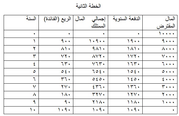
هنا خطتين لتسديد أو استثمار قرض بقيمة (10,000$) لمدة عشر سنوات وبمعدل فائدة (9%)
الخطة الأولى

 ============= الفصل الثالث الاستهلاك ==========
فالسيارة مثلا تنقص قيمتها مع الزمن مهما حاول الإنسان الاعتناء بها فتنقص قيمتها من جراء الاستعمال والتآكل و تتغير طبقا للتحسينات التي تضاف سنويا على السيارات .
إذ يستعمل الاستهلاك لاستعادة قيمة الممتلكات بإحدى الطرق الكثيرة وهو يساعد المحاسبة في معرفة قيمة المشروع النقدي سنة بعد سنة و المبالغ المتبقية من قيمته وهو يبين الطريقة التي تساعد بها تلك المبالغ التي دفعت قيمته للممتلكات ويستعمل الاستهلاك كأساس في كثير من التعاملات مع من يهمهم الأمر , فالحكومة مثلا تضع الضرائب على أرباح الشركات و تضع رقابة على الطريقة التي تستقطع بها مبالغ تغطية رأس المال , مستفيدة من طرق الاستهلاك المختلفة .
أنواع الاستهلاك
ــــــــــــــــــــــــ
التلف بسبب العوامل المحيطة كالرياح و الرطوبة و الحموضة .
التلف بسبب عمل الممتلكات و ينتج عن ذالك تأكلها و تمزقها .
الاستهلاك الوظيفي :- و ينتج بسبب عجز الممتلكات المثابرة في أداء عملها من جراء تغير الطلب عليها و أسبابه :
الهجر :- ويتم الهجر إما لأن هناك آلة في السوق ذات مردود اكبر تحقق ربحا أو لأنه لم يعد من عمل لتلك الآلة
عدم الكفاية :- و يتم هذا عندما تتسع أعمال المنتجين ويحتاجون إلى الآلات ذات استطاعة اكبر .
التفريغ :- يختلف التفريغ عن الاستهلاك الزمني ويتم التفريغ برفع و قطع مادة ما من الممتلكات بصورة مقصودة , أن تفريغ منجم مما فيه من المواد يغير من قيمته و كذالك قطع الأشجار من الغابة ونزح البترول من البئر يقلل من كمية كل منهما .
تقلب مستويات السعر :- إن تغير السعر مع تغير الزمن أمر طبيعي ويؤدي بالتالي إلى تغير قيمة الممتلكات الجديدة و القديمة ومن أسبابه العرض و الطلب و الحروب و الأزمات .
الحوادث و المفاجآت :- للحوادث و المفاجآت اثر سيئ على المشاريع إن لم تتدارك و يحتاط لها فإنها تؤدي إلى خسارة سريعة و كبيرة في القيمة و اعتاد العالم أن يحتاط من هذا الأمر بالتامين في الممتلكات , لآن الحوادث لا يمكن التنبؤ بها و لكن يمكن الإقلال منها بالحيطة و الدراسة و التصميم , فحوادث الحرائق و الانفجار و الاصطدام حوادث رهيبة ومؤلمة , خسائرها فادحة اتخذ حيالها العالم قضية التأمين كحل لها .
طرق حسابه و تقديره :- يحتاج أمر تقدير الاستهلاك إلى خبرة طويلة و إلى معلومات تستقصى من حياة ممتلكات مشابهة استخدمت في ضروف مماثلة اد من الصعب التعرف على قيمة الاستهلاك مقدما بصورة مؤكدة , قد يسهل التعرف على قيمة الاستهلاك المالي و الفيزيائي غير أن التعرف على قيم الاستهلاك الوظيفي عسير إلى حد بعيد .
لذا تقدر مدة الخدمة وقيمة الانقاد للممتلكات , وتجرى حسابات مشابهة استنادا إلى ما هو متوفر من معلومات و إلى خبرة المختصين وحصافتهم عند البدء بتنفيذ المشروع , وتعرف القيمة الغير مغطاة من قيم الممتلكات بقيمة الاستهلاك أو بالقيمة المسجلة أما قيمة الممتلكات في نهاية عمرها الاقتصادي فتسمى بقيمة الانقاد .
--------_____-------
أولا :- الطرق التي تتخذ الزمن أساسا للاستهلاك
--------______--------
1 – طريقة الخط المستقيم : في هذه الطريقة يفرض ان الاستهلاك يتم بانتظام سنويا خلال حياة الموجودات .
==================================
مثال : - آلة قيمتها 14000دولار وقيمة أنقادها 4000 دولار ومدة حياتها عشر سنوات , احسب حمل الاستهلاك والقيمة المسجلة وعوائد رأسمال الغير مغطاة في كل سنة من حياة هذه الآلة , علما بأن الريع المرتجى منها هو (4%) سنويا .
==================================

ـــــــــــــــــــــــــــــــــــــــــــــــ
================
الفصل الرابع
تمويل المشاريع الهندسية
=================
إن تأمين رأس المال لأي مشروع أمر هام و الشروط الذي يحصل بها على رؤوس الأموال ليست متشابهة و لا تحمل نفس القيود و الأشكال ,و لهذا لابد من دراسة مستفيضة للأمر ,ويتألف رأس المال مما يوفره الأشخاص من مكاسبهم أو من فوائد و أرباح ناتجة عن تمويله من مشاريع أخرى
لقد فشل العديد من المشاريع الهندسية لأن السبل أو الطرق التي اخدت منها الأموال اللازمة للمشروع لم تكن بالطرق الملائمة و هذا ما أدى إلى خسارته و توقفه .
فإذا وظف رأس مال في مشروع ما فمن المنتظر أن يؤدي إلى ربح طبقا للدراسات التي بني عليها المشروع و من طرق توفير المال للمشاريع هي الدين فقد يكون رأس المال مستدانا و عندها يقدم المستدين ضمانا على إعادة المبالغ مع فوائدها المقررة ضمن الفترة المحددة .
و قد يمول المشروع بان يقوم جماعة بإصدار أسهم و بيعها بعد أخد موافقة الحكومة على ذالك , هذا النوع من التمويل يدعى بالشركات المساهمة و من هدف هذا التمويل جمع رأس مال اكبر و ضمان لمدة حياة المشروع أطول , ومن الممكن الاستدانة من المصارف و الحكومات لمدة طويلة الأجل.
الشركة
هي عقد يلتزم بمقتضاه شخصين أو اكتر بأن يساهم كل منهم في مشروع يستهدف الربح و ذالك بتقديم حصة من مال أو أعمال وتقاسم ما قد ينشا من المشروع من ربح أو خسارة .
و للشركات أنواع أهمها :
الشركة التضامنية / الشركة المساهمة / شركة التوصية البسيطة /شركة ذات رأس المال القابل للتغيير / شركة ذات المسؤولية المحدودة / شركة ذات التوصية البسيطة / شركة تعاونية /شركة توصية بالأسهم / شركة المحاصصة .
شركة التضامن : هي شركة تتكون من شخصين او اكتر مسؤولين بالتضامن بأموالهم عن ديون الشركة
شروطها :
لا يجوز للشريك فيها أن يتنازل عن حصته ألا بموافقة .
يجب على مدير الشركة إشهار الشركة في الجرائد وتسجيلها في السجل العقاري .
لا يجوز أن تكون حصص الشركاء في الشركة ممثلة بصكوك قابلة للتداول .
لا يجوز للشريك فيها دون موافقة الشركاء أن يمارس نشاط من نوع نشاط الشركة لحسابه او لحساب غيره .
عقد الشركة يضم الأتي :
أسم الشركة و غرضها و مركزها الرئيسي و فروعها إن وجدت .
رأس مال الشركة و تعريف كافي و بالحصص التي تعهد كل شريك بتقديمها .
أسماء الشركاء و مكان إقامتهم و مهنتهم و جنسياتهم .
أسماء المدراء و من لهم حق التوقيع نيابة عن الشركة .
تاريخ تأسيس الشركة و مدتها .
الشركة المساهمة : هي شركة ينقسم فيها رأس المال إلى أسهم متساوية قابلة للتداول و لايسئل الشركاء إلا عن أسهمهم و لا يحوز إن يقل عدد الاسم عن عدد معين و لا يقل سعر السهم عن سعر معين و لا يجور تأسيس شركة مساهمة إلا بموافقة الحكومة و لا يقل رأس المال عن قيمة معينة و لا المدفوع عند التأسيس عن النصف
شركة توصية بالأسهم : و تتكون هذه الشركة من فريقين على الأقل يضم شريك متضامنا مسئولا بأمواله عن ديون الشركة وفريق أخر لا يسألون عن ديون الشركة إلا بمقدار حصته في رأس المال .
شركة رأس المال القابل للتغير : هي شركة ينص عقدها على أن رأس مالها قابل للزيادة أو بانضمام شريك جديد أو قابل للتخفيض من حيت رأس المال أو عدد الشركاء .
الشركة التعاونية : و هي شركة مساهمة تهدف لصالح الشركاء و تقوم على جهودهم للأغراض التالية :
تخفيض قيمة الشراء أو بيع للمنتجات أو الخدمات .
تحسين صنف المنتجات أو مستوى الخدمات .
الأسهم
هي تلك السندات التي تصدرها مجموعة من المؤسسين لشركة اعترافا بمشاركة مساهمين بجزء معين في رأس المال .
هذه الأسهم قد يدون عليها قيمتها و هي القيمة التي بيعت بها لأول مرة و تدعى بالقيمة الاسمية و قد لا يكون لهده القيمة صلة بالقيمة الحقيقية للسهم التي تتغير طبقا لنجاح أو فشل المشروع .
الأسهم أصناف عديدة منها السهم العام و هو السهم الذي يحق لحامله الانتخاب و التصويت على حل الشركة و تغيير قوانينها , وهو يشارك في الأرباح و الخسائر و له حق الاطلاع على سجلات الشركة , ومنها الأسهم المفضلة و هي أسهم ذات مميزات خاصة حيت تضمن لصاحبها أرباحا بنسبة معينة و لا يتحمل أي خسارة تتكبدها الشركة .
قد تحتاج الشركات المساهمة إلى أموال إضافية فتضطر إلى طبع سندات بضمان فائدة معينة لمشتري هذه السندات وهو ما يعرف با السند طويل الأجل و قد تستدين الشركة من احد المصارف لقاء رهن بعض ممتلكاتها كضمان لرد المبلغ و في العادة في مثل هده الحالة لا تزيد مدة القرض عن سنوات محدودة و هو ما يعرف بالدين طويل الأجل و لأصحاب هذه الديون الأسبقية في قبض فوائد ديونهم و لا يتحملون أي خسارة قد تلحق بالشركة ,
و لا يتحل حاملو هده السندات أي مسؤولية اتجاه الشركة و ليس لهم الحق في التصويت أو الانتخاب .
تصنيف السندات
سندات ضد الممتلكات : و ضمان هذه الأسهم هو ممتلكات الشركة التي توضع كضمان لقيمة السند المباع
سندات متعلقة : و يكون ضمان هده الأسهم سندات أخرى أو أسهم أخرى عائدة إلى مشروع أخر ناجح
سندات الاعتماد : و تصدر هده السندات شركات ذات السمعة الطيبة واسعة الانتشار وتكون سندات مضمونة و عليها طلب كبير.
مما سبق يتبن أن حامل السهم هو شريك في الأرباح و يتحمل الخسائر و له كل المميزات و الحقوق و عليه الواجبات أما حامل السند ما هو إلا دائن للمشروع و لا يترقب من المشروع إلا الحصول على فائدة محدودة خلال مدة السند بالإضافة إلى استعادة مبلغه كاملا دون زيادة أو نقصان عند شراء السند .
ابوبكر عبد الوهاب
إبراهيم صالح ابونوارة
=====================
الشرح التالى باللغة الانجليزية لمادة الاقتصاد الهندسى
نقلا عن موقع
http://www.isr.umd.edu
:::::::::::::::::::::::::::::::::::
INTRODUCTION
WHY DO ENGINEERS NEED TO LEARN ABOUT ECONOMICS?
Ages ago, the most significant barriers to engineers were technological. The things that engineers wanted to do, they simply did not yet know how to do, or hadn't yet developed the tools to do. There are certainly many more challenges like this which face present-day engineers. However, we have reached the point in engineering where it is no longer possible, in most cases, simply to design and build things for the sake simply of designing and building them. Natural resources (from which we must build things) are becoming more scarce and more expensive. We are much more aware of negative side-effects of engineering innovations (such as air pollution from automobiles) than ever before.
For these reasons, engineers are tasked more and more to place their project ideas within the larger framework of the environment within a specific planet, country, or region. Engineers must ask themselves if a particular project will offer some net benefit to the people who will be affected by the project, after considering its inherent benefits, plus any negative side-effects (externalities), plus the cost of consuming natural resources, both in the price that must be paid for them and the realization that once they are used for that project, they will no longer be available for any other project(s).
Simply put, engineers must decide if the benefits of a project exceed its costs, and must make this comparison in a unified framework. The framework within which to make this comparison is the field of engineering economics, which strives to answer exactly these questions, and perhaps more. The Accreditation Board for Engineering and Technology (ABET) states that engineering "is the profession in which a knowledge of the mathematical and natural sciences gained by study, experience, and practice is applied with judgment to develop ways to utilize, economically, the materials and forces of nature for the benefit of mankind".1
It should be clear from this discussion that consideration of economic factors is as important as regard for the physical laws and science that determine what can be accomplished with engineering. The following figure shows how engineering is composed of physical and economic components:
![[Eng. Economics]](http://www.isr.umd.edu/%7Eaustin/ence202.d/economics-fig1.gif)
Figure 1 shows how engineering is composed of physical and economic components.
- Physical Environment : Engineers produce products and services depending on physical laws (e.g. Ohm's law; Newton's law).
Physical efficiency takes the form:
                                    system output(s)
      Physical (efficiency )  =  -------------------
system input(s) - Economic Environment : Much less of a quantitative nature is known about economic environments -- this is due to economics being involved with the actions of people, and the structure of organizations.
Satisfaction of the physical and economic environments is linked through production and construction processes. Engineers need to manipulate systems to achieve a balance in attributes in both the physical and economic environments, and within the bounds of limited resources. Following are some examples where engineering economy plays a crucial role:
- Choosing the best design for a high-efficiency gas furnace
- Selecting the most suitable robot for a welding operation on an automotive assembly line
- Making a recommendation about whether jet airplanes for an overnight delivery service should be purchased or leased
- Considering the choice between reusable and disposable bottles for high-demand beverages
With items 1 and 2 in particular, note that coursework in engineering should provide sufficient means to determine a good design for a furnace, or a suitable robot for an assembly line, but it is the economic evaluation that allows the further definition of a best design or the most suitable robot.
In item 1 of the list above, what is meant by " high-efficiency"? There are two kinds of efficiency that engineers must be concerned with. The first is physical efficiency, which takes the form:
                                  System output(s)
      Economic (efficiency )  =  -----------------
                                 System input(s)
For the furnace, the system outputs might be measured in units of heat energy, and the inputs in units of electrical energy, and if these units are consistent, then physical efficiency is measured as a ratio between zero and one. Certain laws of physics (e.g., conservation of energy) dictate that the output from a system can never exceed the input to a system, if these are measured in consistent units. All a particular system can do is change from one form of energy (e.g. electrical) to another (e.g., heat). There are losses incurred along the way, due to electrical resistance, friction, etc., which always yield efficiencies less than one. In an automobile, for example, 10-15% of the energy supplied by the fuel might be consumed simply overcoming the internal friction of the engine. A perfectly efficient system would be the theoretically impossible Perpetual Motion Machine!
The other form of efficiency of interest to engineers is economic efficiency, which takes the form:
                                    system worth
      Economic (efficiency )  =  -----------------
                                   system cost
You might have heard economic efficiency referred to as "benefit-cost ratio". Both terms of this ratio are assumed to be of monetary units, such as dollars. In contrast to physical efficiency, economic efficiency can exceed unity, and in fact should, if a project is to be deemed economically feasible. The most difficult part of determining economic efficiency is accounting for all the factors which might be considered benefits or costs of a particular project, and converting these benefits or costs into a monetary equivalent. Consider for example a transportation construction project which promises to reduce everyone's travel time to work. How do we place a value on that travel time savings? This is one of the fundamental questions of engineering economics.
In the final evaluation of most ventures, economic efficiency takes precedence over physical efficiency because projects cannot be approved, regardless of their physical efficiency, if there is no conceived demand for them amongst the public, if they are economically infeasible, or if they do not constitute the "wisest" use of those resources which they require.
There are numerous examples of engineering systems that have physical design but little economic worth (i.e it may simply be too expensive !!). Consider a proposal to purify all of the water used by a large city by boiling it and collecting it again through condensation. This type of experiment is done in junior physical science labs every day, but at the scale required by a large city, is simply too costly.
ROLE OF UNCERTAINTY IN ENGINEERING
When conducting engineering economic analyses, it will be assumed at first, for simplicity, that benefits, costs, and physical quantities will be known with a high degree of confidence. This degree of confidence is sometimes called assumed certainty. In virtually all situations, however, there is some doubt as to the ultimate values of various quantities. Both risk and uncertainty in decision-making activities are caused by a lack of precise knowledge regarding future conditions, technological developments, synergies among funded projects, etc. Decisions under risk are decisions in which the analyst models the decision problem in terms of assumed possible future outcomes, or scenarios, whose probabilities of occurrence can be estimated. Of course, this type of analysis requires an understanding of the field of probability. Decisions under uncertainty, by contrast, are decision problems characterized by several unknown futures for which probabilities of occurrence cannot be estimated. Other less objective means exist for the analysis of such problems.
For the purposes of this brief tutorial, we cannot delve further into the analytical extensions required to accommodate risk or uncertainty in the decision process. We must recognize that these things exist, however, and be careful about reaching strong conclusions based on data which might be susceptible to these. Because engineering is concerned with actions to be taken in the future, an important part of the engineering process is improving the certainty of decisions with respect to satisfying the objectives of engineering applications.
THE ENGINEERING PROCESS
Engineering activities dealing with elements of the physical environment take place to meet human needs that arise in an economic setting. The engineering process employed from the time a particular need is recognized until it is satisfied may be divided into a number of phases:
- Determination of Objectives
This step involves finding out what people need and want that can be supplied by engineering. People's wants may arise from logical considerations, emotional drives, or a combination of the two.
- Identification of Strategic Factors
The factors that stand in the way of attaining objectives are known as limiting factors. Once the limiting factors have been identified, they are examined to locate strategic factors -- those factors which can be altered to remove limitations restricting the success of an undertaking. A woman who wants to empty the water from her swimming pool might be faced with the limiting factor that she only has a bucket to do the job with, and this would require far greater time and physical exertion than she has at her disposal. A strategic factor developed in response to this limitation would be the procurement of some sort of pumping device which could do the job much more quickly, with almost no physical effort on the part of the woman.
- Determination of means (engineering proposals)
This step involves discovering what means exist to alter strategic factors in order to overcome limiting factors. In the previous example, one means was to buy (or rent) a pump. Of course, if the woman had a garden hose, she might have been able to siphon the water out of the pump. In other engineering applications, it may be necessary to fabricate the means to solve problems from scratch.
- Evaluation of Engineering Proposals
It is usually possible to accomplish the same result with a variety of means. Once these means have been described fully, in the form of project proposals, economic analysis can be employed to determine which among them, if any, is the best means for solving the problem at hand.
- Assistance in Decision Making
It is commonplace for the final decision-making responsibility to fall on the head(s) of someone other than the engineer(s). The person(s) so charged, however, may not be sufficiently knowledgeable about the technical aspects of a proposal to determine its relevant worth compared to other means. The engineer can help to bridge this gap.
ENGINEERING ECONOMIC STUDIES
The four key steps in planning an economic study are :
- Creative Step : People with vision and initiative adopt the premise that better opportunities exist than are known to them. This leads to research, exploration, and investigation of potential opportunities.
- Definition Step : System alternatives are synthesised with economic requirements and physical requirements, and enumerated with respect to inputs/outputs.
- Conversion Step : The attributes of system alternatives are converted to a common measure so that systems can be compared.
Future cash flows are assigned to each alternative, consisting of the time-value of money.
- Decision Step : Qualitative and quantitative inputs and outputs to/from each system form the basis for system comparison and decision making. Decisions among system alternatives should be made on the basis of their differences. For a small number of real world systems there will be complete knowledge. All facts/information and their relationships, judgements and predictive behavior become a certainty. For most systems, however, even after all of the data that can be bought to bear on it has been considered, some areas of uncertainty are likely to remain. If a decision must be made, these areas of uncertainty must be bridged by consideration of non-quantitative data/information, such as common sense, judgement and so forth.
Decisions among system alternatives should be made on the basis of their differences.
For a small number of real world systems there will be complete knowledge. Dll facts/information and their relationships, judgements and predictive behavior become a certainty.
For most systems, however, even after all of the data that can be bought to bear on it has been considered, some areas of uncertainty are likely to remain. If a decision must be made, these areas of uncertainty must be bridged by consideration of non-quantitative data/information, such as common sense, judgement and so forth.
Examples :
- Infrastructure expenditure decision
- Replace versus repair decisions
- Selection of inspection method
- Selection of a replacement for an equipment
FUNDAMENTAL ECONOMIC CONCEPTS
Economics deals with the behavior of people, and as such, economic concepts are usually qualitative in nature, and not universal in application.
UTILITY
- Utility is the power of a good or service to satisfy human needs.
VALUE
- Designates the worth that a person attaches to an object or service.
- Is a measure or appraisal of utility in some medium of exchange.
- Is not the same as cost or price.
CONSUMER AND PRODUCER GOODS
- Consumer goods : Consumer goods are the goods and services that directly satisfy human wants. For example, TV, shoes, houses.
- Producer goods : Producer goods are the goods and services that satisfy human wants indirectly as a part of the production or construction process. For example, factory equipment, industrial chemicals ands materials.
UTILITY OF GOODS
- Consumer goods : Basic human needs of food, clothing and shelter. In commercial advertisements, emphasis is given to senses not reasoning. The utility in this case is considered objectively and/or subjectively.
- Producer goods : The utility stems for their means to get to an end. The utility in this case is considered objectively.
ECONOMY OF EXCHANGE
- Occurs when utilities are exchanged by two or more people.
- It is possible because consumer utilities are evaluated subjectively.
- Represents mutual benefit in exchange.
- Persuasion in exchange. Salesperson.
ECONOMY OF ORGANIZATION
Through organizations, ends can be attained or attained more economically by:
- Labor saving
- Efficiency in manufacturing or capital use
CLASSIFICATION OF COST
A key objective in engineering applications is the satisfaction of human needs, which will nearly always imply a cost.
Economic analyses may be based on a number of cost classifications:
- First (or Initial) Cost : Cost to get activity started such as property improvement, transportation, installation, and initial expenditures.
- Operation and Maintenance Cost : They are experienced continually over the usefull life of the activity.
- Fixed Cost : Fixed costs arise from making preparations for the future, and includes costs associated with ongoing activities throughout the operational life-time of that concern. Fixed costs are relatively constant; they are decoupled from the system input/output, for example.
- Variable Cost : Variable costs are related to the level of operational activity (e.g. the cost of fuel for construction equipment will be a function of the number of days of use).
- Incremental or Marginal Cost : Incremental (or marginal) cost is the additional expense that will be incurred from increased output in one or more system units (i.e. production increase). It is determined from the variable cost.
- Sunk Cost : It cannot be recovered or altered by future actions. Usually this cost is not a part of engineering economic analysis.
- Life-Cycle Cost : This is cost for the entire life-cycle of a product, and includes feasibility, design, construction, operation and disposal costs.
SUPPLY AND DEMAND (not covered)
- Demand curve shows the number of units people are willing to buy and cost per unit (decreasing curve).
- Supply curve shows the number of units that vendors will offer for sale and unit price (increasing curve).
- The intersection defines the exchange price.
- Elasticity of demand. Price changes and their effect on demand changes. It depends on whether the consumer product is a necessity or a luxury.
- Law of diminishing return. A process can be improved at a rate with a diminishing return. Example: cost of inspection to reduce cost of repair and lost production.
INTEREST RATE
Interest is a rental amount charged by financial institutions for the use of money.
- Called also the rate of capital growth, it is the rate of gain received from an investment.
- It is expressed on an annual basis.
- For the lender, it consists, for convenience, of (1) risk of loss, (2) administrative expenses, and (3) profit or pure gain.
- For the borrower, it is the cost of using a capital for immediately meeting his or her needs.
TIME VALUE OF MONEY
The time-value of money is the relationship between interest and time. i.e.
![[Time-Value of Money]](http://www.isr.umd.edu/%7Eaustin/ence202.d/economics-fig2.gif)
Money has time-value because the purchasing power of a dollar changes with time.
EARNING POWER OF MONEY
The earning power of money represents funds borrowed for the prospect of gain.
Often these funds will be exchanges for goods, services, or production tools, which in turn can be employed to generate and economic gain.
PURCHASING POWER OF MONEY
The prices of goods and services can go upward or downward, and therefore, the purchasing power of money can change with time.
- Price Reductions : Caused by increases in productivity and availability of goods.
- Price Increases : Caused by government policies, price support schemes, and deficit financing.
EXAMPLE ECONOMIC STUDIES
- Design and Economy
- Elimination of overdesign should not be an objective.
- Designing for economic production
- Economy in the design of producer goods
- Design for the economy of maintenance
- Design for the economy of shipping
- Economy of interchangeable design
Economy of Material Selection
Standardization and Simplification
- Selection of Personnel
- Range of human capacities
- Range of human capacities
- Economy of proficiency
- Economy of specialization
- Economy of dependability
Economy of Resource Input for Organizations
- Tangible versus intangible inputs and their evaluations
Knowledge and Information
- Tangible versus intangible inputs and their evaluations Qualitative versus quantitative
CASH FLOW DIAGRAMS
The diagram convention is as follows:
- Horizontal Axis : The horizontal axis is marked off in equal increments, one per period, up to the duration of the project.
- Revenues : Revenues (or receipts) are represented by upward pointing arrows.
- Disbursements : Disbursements (or payments) are represented by downward pointing arrows.
Arrow lengths are approximately proportional to the magnitude of the cash flow.
Expenses incurred before time = 0 are sunk costs, and are not relevant to the problem.
![[Cash Flows]](http://www.isr.umd.edu/%7Eaustin/ence202.d/economics-fig3.gif)
- Cash Flow over Time : Upward arrow means positive flow, downward arrow means negative flow. There are two cash flows to each problem (borrower and lender flows).
- Net Cash Flow : The arithmetic sum of receipts (+) and disbursements (-) that occur at the same point in time.
INTEREST FORMULAE
Interest formulae play a central role in the economic evaluation of engineering alternatives.
TYPES OF INTEREST
- Simple Interest : I = Pni.
     P = Principal
    i = Interest rate
    n = Number of years (or periods)
    I = Interestt.
Interest is due at the end of the time period. For fractions of a time period, multiply the interest by the fraction.Example : Suppose that $50,000 is borrowed at a simple interest rate of 8% per annum. At the end of two years the interest owed would be:
    I = $ 50,000 * 0.08 * 2
= $ 8,000 - Compound Interest : The interest of the interest.
Example : A loan of $1,000 is made at an interest of 12% for 5 years. The interest is due at the end of each year with the principal is due at the end of the fifth year. The following table shows the resulting payment schedule:Principal P = $1000.00
Interest Rate i = 0.12.
Number of years (or periods) n = 5.
================================================================
Amount at Interest at Owed amount at
Year start of year end of year end of year Payment
================================================================
1 $1000.00 $120.00 $1120.00 $120.00
2 $1000.00 $120.00 $1120.00 $120.00
3 $1000.00 $120.00 $1120.00 $120.00
4 $1000.00 $120.00 $1120.00 $120.00
5 $1000.00 $120.00 $1120.00 $120.00
Example : A loan of $1,000 is made at an interest of 12% for 5 years. The principal and interest are due at the end of the fifth year. The following table shows the resulting payment schedule:Principal P = $1000.00
Interest Rate i = 0.12.
Number of years (or periods) n = 5.
================================================================
Amount at Interest at Owed amount at
Year start of year end of year end of year Payment
================================================================
1 $1000.00 $120.00 $1120.00 $0.00
2 $1120.00 $134.40 $1254.40 $0.00
3 $1254.40 $150.53 $1404.93 $0.00
4 $1404.93 $168.59 $1573.52 $0.00
5 $1573.52 $188.82 $1762.34 $1762.34
INTEREST FORMULAE (Discrete Compounding and Discrete Payments)
Notations:
    i = The annual interest rate
   n = The number of annual interest periods
   P = A present principal sum
   A = A single payment, in a series of n equal payments, made at the end
       of each annual interest period
   F = A future sum, n annual interest periods hence
- Single-Payment Compound-Amount Factor
F = P.[1 + i]^n
Example 1 : Let the principal P = $1000, the interest rate i = 12%, and the number of periods n = 4 years. The future sum is:
    F = $1000 [1 + 0.12] ^ 4
= $1,573.5![[Single Payment]](http://www.isr.umd.edu/%7Eaustin/ence202.d/economics-fig6.gif)
Figure 4 : Cash Flow for Single Payment Compound Amount Figure 4 shows the cash flow for the single present amount (i.e. P = 1000) and the single future amount (i.e. F = $1,573.5).
- Single-Payment Present-Worth Factor
            F
   P = =========
       [1 + i]^n
The factor 1.0/[ 1 + i ]^n is known as the single-payment present-worth factor, and may be used to find the present worth P of a future amount F.
Example 1 : Let the future sum F = $1000, interest rate i = 12%, and number of periods n = 4 years. The single payment present-worth factor is:
            F           $1000.00
   P = =========  =  ==============  =   $635.50.
       [1 + i]^n     [ 1 + 0.12 ]^4
The present worth P = $635.50.
Example 2 : Let the future sum F = $1,573.5, the interest rate i = 12%, and the number of periods n = 4 years. The single payment present-worth factor is:
            F           $1573.50
   P = =========  =  ==============  =  $1000.00.
       [1 + i]^n     [ 1 + 0.12 ]^4
The present worth P = $1000.00.
- Equal Payment-Series Compound Amount Factor
Some economic studies require the computation of a single factor value that would accumulate from a series of payments occurring at the end of succeeding interest periods.
![[Compound Amounts]](http://www.isr.umd.edu/%7Eaustin/ence202.d/economics-fig4.gif)
Figure 5 : Schematic of Equal Payment-Series Compount Amounts Figure 5 represents this scenario in graphical terms. At the end of Year 1 a payment of $ A begins the accumulation of interest at rate i% for (n-1) years. At the end of Year 2 a payment of $ A begins the accumulation of interest at rate i% for (n-2) years. End of year payments of $ A continue until Year N (or n as written below).
The total accumulatio of funds at Year N is simply the sum of $A payments multiplied by the appropriate single-payment present-worth factors. In tabular format we have:
    End of             Compound Amount at                Total
     Year             the end of n Years      Compound Amount
   ==========================================================
        1      $ A . [ 1 + i ] ^ (n - 1)
        2      $ A . [ 1 + i ] ^ (n - 2)
        3      $ A . [ 1 + i ] ^ (n - 3)

    n - 1      $ A . [ 1 + i ]
        n      $ A
   ==========================================================
                                                          $ F
   ==========================================================
The total compound amount is simply the sum of the compound amounts for years 1 though n. This sumation is a geometric series:
F = A + A.[1 + i] + A.[1+i]^2 + ..... + A.[1+i]^(n-1)
With a little bit of mathematical manipulation, it can be shown;
            [ 1 + i ]^n - 1
   F = A * ---------------
                 i
Example 1: Let A = 100, i = 12%, and n = 4 years.
              [ 1 + 0.12 ]^4 - 1
   F = 100 * ------------------ = 477.9
0.12 - Equal-Payment Series Sinking-Fund Factor
Given a future amount F, the equal payments compound-amount relationship is:
                  i
   A = F * ---------------
           [ 1 + i ]^n - 1
A = required end-of-year payments to accumulate a future amount F.
Example 1: Let F = 1000, i = 12%, and n = 4 years.
                     0.12
   A = 1000 * ------------------ = 209.2
[ 1 + 0.12 ]^4 - 1 - Equal-Payment-Series Capital-Recovery Factor
A deposit of amount P is made now at an interest rate i. The depositor wishes to withdraw the principal plus earned interest in a series of year-end equal payments over N years, such that when the last withdrawl is made there should be no funds left in the account.
![[Capital Recovery]](http://www.isr.umd.edu/%7Eaustin/ence202.d/economics-fig5.gif)
Figure 6 : Schematic of Equal-Payment-Series Capital Recovery Figure 6 summarizes the flow of disbursements and receipts (from the depositors point of view) for this scenario.
Equating the principle $P (plus accumulated interest) with the accumulation of equal payments $A (plus appropriate interest) gives:
                        [ [ 1 + i ]^n - 1 ]
   P [ 1 + i ]^n  = A  -------------------
                               i
which can be rearranging to give:
            i * [ 1 + i ]^n
   A = P * ---------------
           [ 1 + i ]^n - 1
This is the case of loans (mortgages).
Example 1: Let P = 1000, i = 12%, and n = 4 years
                0.12 * [ 1 + 0.12 ]^4
   A = $1000 * --------------------- = $329.2
[ 1 + 0.12 ]^4 - 1 - Equal-Payment-Series Present-Worth Factor
This can be described as
            [ 1 + i ]^n - 1
   P = A * ---------------
           i * [ 1 + i ]^n
Example 1: Let A = 100, i = 12%, and n = 4 years.
              [ 1 + 0.12 ]^4 - 1
   P = 100 * --------------------- = 303.7
0.12 * [ 1 + 0.12 ]^4 - Uniform Gradient-Series Factor
Often periodic payments do not occur in equal amounts, and may increase or decrease by constant amounts (e.g. $100, $120, $140, $160 .... $200).
The gradient (G) is a value in the cash flow that starts with 0 at the end of year 1, G at the end of year 2, 2G at the end of year 3, and so on to (n-1)G at the end of year n.
This can be described as
            *-                      -*
           |  1          n          |
   A = G . |  - -  ---------------  |
           |  i    [ 1 + i ]^n - 1  |
           *-                      -*
Example 1 : Let G = 100, i = 12%, and n = 4 years.
               *-                           -*
              |    1          4             |
   A = $100 . |  ---- -  ------------------ | = $ 135.9
              |  0.12    [ 1 + 0.12 ]^4 - 1 |
              *-                           -*
DISCRETE AND CONTINUOUS COMPOUNDING (compounding frequency)
Nominal interest rate : is expressed on an annual basis. Financial institutions refer to this rate as annual percentage rate (APR).
Effective interest rate : is an interest rate that is compounded using a time period less than a year. The nominal interest rate in this case is the effective rate times the number of compounding periods in a year. Then, it is referred to as nominal rate compounded at the period less than a year.
Example : If the effective rate is 1% per month, it follows that the nominal rate is 12% compounded monthly.
Relationship between the two rates. Let's define:
    r = nominal interest rate per year
   i = effective interest rate in the time interval
   l = length of the time interval (in years)
   m = reciprocal of the length of the compounding period (in years)
Therefore, the effective interest rate for any time interval is given by:
         *-         -* ^ l*m
        |       r   |
   i =  |  1 + ---  |     -    1.0
        |       m   |
        *-         -*
Clearly if l*m = 1, then i is simply r/m.
The product l*m is called c = the number of compounding periods in the time interval l. Note that c should be > 1.
Continuous compounding: The limiting case for the effective rate is when compounding is performed an infinite times in a year, that is continuously. Using l = 1, the following limit produces the continuously compounded interest rate
                       *-         -* ^ m
                      |       r   |
   i_a =        Limit |  1 + ---  |   -  1.0
          m->infinity |       m   |
                      *-         -*
resulting into and effective interest rate
i_a = e^r - 1
Example :
 ================================================================
 Compounding    Number of   Effective interest  Effective annual
   frequency      Periods      rate per period     interest rate
================================================================

    Annually          1.0                  18%            18.00%
Semiannually          2.0                   9%            18.81$
   Quarterly          4.0                 4.5%            19.25%
     Monthly         12.0                 1.5%            19.56%
      Weekly         52.0              0.3642%            19.68%
       Daily        365.0              0.0493%            19.74%
Continuously     infinity              0.0000%            19.72%
Interest Formulas (Continuous Compounding and Discrete Payments)
Interest Formulas (Continuous Compounding and Continuous Payments)
Handout. (Table)
ECONOMIC EQUIVALENCE INVOLVING INTEREST
Why? It is common in engineering to compare alternatives.
THE MEANING OF EQUIVALENCE
In engineering economy two things are said to be equivalent when they have the same effect. Unlike most individual involved with personal finance, industrial decision makers using engineering economics are not so much concerned with the timing of a project's cash flows as with the profitability of that project. This means that mechanisms are needed to compare projects involving receipts and disbursements occurring at different times, with the goal of identifying an alternative having the largest eventual profitability [Lindeberg82].
EQUIVALENCE CALCULATIONS INVOLVING A SINGLE FACTOR
The interest equations are affected by three factors: (a) amounts, (b) times of occurrence of amounts, and (c) rate of interest.
- Single-Payment Compound-Amount Factor
F = P.[1 + i]^n
Example 1 : Let P = $1000, i = ??, n = 4 years, and F = $1200. The interest rate is
F = $1200.00 = $1000.00 [1 + i ]^4
Rearranging terms in this equation gives i = 1.2^0.25 - 1 = 0.046635.
Example 2 : Let P = $1000, i = 10%, n = ?? years, and F = $1200.
F = $1200.00 = $1000.00 [1 + 0.10 ]^n
Rearranging terms in this equation gives n = 1.91 years.
- Single-Payment Present-Worth Factor
            F
   P = ---------
       [1 + i]^n
Example 1 : Let F = $1000, i = 12%, n = 4 years, and P = ?
          $1000.00
   P = ------------ = $635.5
[1 + 0.12]^4 - Equal-Payment-Series Compound-Amount Factor
            [ 1 + i ]^n - 1
   F = A * ---------------
                 i
The derivation of this formula can be found on page 46 of the economics text.
Example 1 : Let A = $100.00, i = 10%, and F = $1000.00. How many years n are needed ?
                         [ 1 + 0.12 ]^n - 1
   $1000.00 = $100.00 * ------------------
                              0.12
Rearranging the terms in this equation gives n = 7.27 years.
- Equal-Payment-Series Sinking-Fund Factor
                  i
   A = F * ---------------
           [ 1 + i ]^n - 1
Example 1 : Paying towards a future amount. Let F = $1000.00, i = 12%, and n = 4 years. What is A ?
                         0.12
   A = $1000.00 * ------------------ = $209.20
[ 1 + 0.12 ]^4 - 1 - Equal-Payment-Series Capital-Recovery Factor
            i * [ 1 + i ]^n
   A = P * ---------------
           [ 1 + i ]^n - 1
Example 1 : Paying back a loan. Let P = $1000, i = 12%, n = 4 years, and A = ?
               0.12 * [ 1 + 0.12 ]^4
   A = 1000 * --------------------- = 329.2
[ 1 + 0.12 ]^4 - 1 - Equal-Payment-Series Present-Worth Factor
            [ 1 + i ]^n - 1
   P = A * ---------------
           i * [ 1 + i ]^n
Example 1 : Let A = 100, i = 10%, and n = 8 years.
                [ 1 + 0.10 ]^8 - 1
   P = 100 * ---------------------- = 533.49
0.10 * [ 1 + 0.10 ]^8 - Uniform Gradient-Series Factor
As explained above, the gradient (G) is a value in the cash flow that starts with 0 at the end of year 1, G at the end of year 2, 2G at the end of year 3, and so on to (n-1)G at the end of year n.
This can be described as
        *-                      -*
       |  1          n          |
A = G . |  - -  ---------------  |
       |  i    [ 1 + i ]^n - 1  |
       *-                      -*
Example 1 : Let G = 100, i = 12%, n = 4 years, and A = ??
        *-                            -*
       |    1             4           |
A = 100.|  ---- -  ------------------  | = 135.9.
       |  0.12    [ 1 + 0.12 ]^4 - 1  |
       *-                            -*
EQUIVALENCE CALCULATIONS INVOLVING CASH FLOW
Two cash flows need to be presented along the same time period using a similar format to facilitate comparison.
When interest is earned, monetary amounts can be directly added only if they occur at the same point in time.
EQUIVALENCE BETWEEN CASH FLOWS
Equivalent cash flows are those that have the same value.
Example : Two equivalent cash flows.
     Cash Flow 1                          Cash Flow 2
=====================================================
   P = $1000.00                            P = $0.00
        i = 12%                              i = 12%
    n = 4 years                          n = 4 years
      F = $0.00    F = $$1000*[1+0.12]^4 = $1,573.50
The equivalence can be established at any point in time. Arbitrarily setting n = 8 years, for example, gives:
For cash flow 1 : F = $1000.0 * [1 + 0.12]^8 = $2475.96
For cash flow 2 : F = $1573.5 * [1 + 0.12]^4 = $2475.96
Note : Two or more distinct cash flows are equivalent if they are equivalent to the same cash flow.
EQUIVALENCE FOR DIFFERENT INTEREST RATES
Example 1 : Given the following cash flow:
===================================================
                          Interest rate applicable
                          from previous year (t-1)
Year End        Amount      to current year end (t)
===================================================
      0         $0.00                           NA
      1       $200.00     12% compounded quarterly
      2         $0.00     12% compounded quarterly
      3       $100.00       7% compounded annually
      4       $100.00      10% compounded annually
      5       $100.00      10% compounded annually
The above cash flow can be converted to its present value as follows:
Assuming the following cash flow:
===================================================
Time (Year End)     Receipts          Disbursements
===================================================
            0         $0.00              -$1000.00
            1         $0.00               -$500.00
            2       $482.00                  $0.00
            3       $482.00                  $0.00
            4       $482.00                  $0.00
            5         $0.00               -$250.00
            6       $482.00                  $0.00
            7       $482.00                  $0.00
In this case, equivalence states that the actual interest rate earned on an investment is the one that sets the equivalent receipts to the equivalent disbursements.
For the above table, the following equality can be set:
    $1000 + $500.00 (P/F,i,1) + $250(P/F,i,5) =
   $482(P/A,i,3)(P/F,I,1) + $482.00 (P/A,i,2)(P/F,i,5)
By trial and error i = 10% will make the above equation valid. The equivalence can be made at any point of reference in time, it does not need to be the origin (time = zero) to produce the same answer.
If the receipts and disbursement of cash flow are equivalent for some inter= est rate, the cash flows of any equivalent portion of the investment are eq= ual at that interest rate to the negative (-) of the equivalent amount of t= he cash flows that constitute the remaining portion on the investment.
For example, break-up the above cash flow between year 4 and 5. Perform th= e equivalence at the 4th year produces the following:
-1000(F/P,10,4)-500(F/P10,3)+482(F/A,10,3) = -(-250(P/F,10,1)+482(P/A,10,2)(P/F,10,1))

-1000(1.464)-500(1.331)+482(3.310) =  -$(-250(0.9091)+482(1.7355)(0.9091))
                            -$534 = -$534
EQUIVALENCE CALCULATIONS WITH MORE FREQUENT COMPOUNDS
- Compounding and Payment Periods Coincide
Assume for example that
Interest = 10% compounded semiannually => 5% per semiannual period
Payments are done semiannually for three years => 3(2) = 6 periods
The calculations from here on are the same as before.
- Compounding More Frequent than Payments
- Calculations based on the compounding period:
Example 1 : Payments = 100 at year end for three years; Interest = 6% per year compounded quarterly.
    i = 6/4 = 1.25%
   F = $100 (F/P,1.25,8) + $100 (F/P,1.25,4) + $100
= $318.8 - Effective interest rate for l = 1 year,
     *-         -*^l       *-         -*^4
    |       r   |         |       6   |
i =  |  1 + ---  | - 1  =  |  1 + ---  |  - 1 = 6.14%
    |       m   |         |       4   |
    *-         -*         *-         -*
The solution of the previous example is
F = $100 (F/A,6.14,3) = $318.80
Example 2 : Assume that end of month payments = 100 with interest of 15% continuous compounding. What is the accumulated amount after 5 years ? The number of periods =12*5 = 60 years. The interest per month is 1/12= 1.25%. Then,
         *-          -*             *-                -*
        | e^(rn) - 1 |             |  e^0.0125*60 - 1 |
  F = A | ---------- | = $100.00 * |  --------------- | = $8,865
        | e^r -1     |             |  e^0.0125 - 1    |
        *-          -*             *-                -*
- Calculations based on the compounding period:
- Compounding Less Frequent than Payments
Usually no interest is paid for funds deposited during an interest period. In this case, funds earn interest after completing the next interest period.
BOND PRICES AND INTEREST
Suppose you can buy a bond for $900 that has a face value of $1000 with 6% annual interest that is paid semiannually. The bond matures in 7 years. The yield to maturity is defied as the rate of return on the investment for its duration. Using equivalence, the following expression can be developed:
$900 = $30 (P/A,i,14) + $1000 (P/F,i,14)
By trial and error, it can be determined that i = 3.94% per semiannual period.
The nominal rate is 2(3.94) = 7.88%.
The effective rate is 8.04%.
The bond market.
EQUIVALENCE CALCULATIONS FOR LOANS
The effective interest rate for a loan is defines as the rate that sets the= receipts equal to the disbursements on an equivalent basis.
REMAINING BALANCE OF A LOAN
Suppose a five-year loan of $10,000 (with interest of 16% compounded quarterly with quarterly payments) is to be paid off after the 13th payment. What is the balance?
The quarterly payment is
$10,000 (A/P,4,20) = $10.000 (0.0736) = $736.00
The balance can be based on the remaining payments as
$736 (P/A,4,7) = $736 * (6.0021) = $4418.
PRINCIPAL AND INTEREST PAYMENTS
Consider the case of a loan with fixed rate and constant payment A. Define the following:
    I_t = Interest payment of A at time t.
   B_t = Portion of payment of A to reduce balance at time t.
     A = I_t + B_t  for t = 1, 2, ....  n
The balance at end of (t-1) is given by => A(P/A,i,n-(t-1)).
Therefore,
    I_t = A(P/A,i,n-(t-1))(i)
   B_t = A - I_t
       = A[1-(P/A,i,n-(t-1))(i)]
Since
P/F,i,n = 1 - (P/A,i,n)(i) => B_t = A(P/F,i,n-t+1)
Example : For P = $1000.00 (loan), n = 4, and i = 15%, the following table can be constructed:
The payment is A = $1000(A/P,15,4) = $1000(0.3503) = $350.30
===============================================================
   Year       Loan                                    Interest
    End    Payment          Payment on Principal       Payment
===============================================================
      1    $350.30   $350.30(P/F,15,4) = $200.30       $150.00
      2    $350.30                       $230.32       $119.98
      3    $350.30                       $264.90        $85.40
      4    $350.30                       $304.62        $45.68
  TOTAL   $1401.12                      $1000.14       $401.06
ECONOMIC EQUIVALENCE INVOLVING INFLATION
MEASURE OF INFLATION AND DEFLATION
The price index is the ratio between the current price of a commodity or service to the price at some earlier reference time. For example, the base year is 1967 (index =100), and the commodity price is $1.46/lb.
The price in 1993 is $5.74/lb.
Therefore, the 1993 index is 5.74/1.4 = 393.2
Note : Actual Consumer price index (CPI) and annual inflation rates for 1965 are shown in Table 5.1 of the Economics Text.
ANNUAL INFLATION RATE
The annual inflation rate at t+1 can be computed as
         CPI(t+1) - CPI(t)
        -----------------
             CPI(t)
Assume the average inflation rate = f. The average rate can be computed as
CPI(t) [ 1 + f ] ^ n = CPI(t+n)
Example : Let the CPI(1966) = 97.2 and the CPI(1980) = 246.80. The average rate of inflation over the 14 year interval is:
        *-        -* ^ (1/14)
       |  246.80  |
   f = | -------- |     -     1.0  =  6.88% per year.
       |  97.2    |
       *-        -*
PURCHASING POWER OF MONEY
Purchasing power at time t in reference to time t-n is
         CPI(t-n)
        --------
        CPI(t)
Now let's define k = annual rate of loss in purchasing power. Therefore the average rate of loss of purchasing power is
CPI(t+n) [ 1 - k] ^ n = CPI(t)
It follows that
                           1
       [ 1 + f ]^n = -----------
                     [ 1 - k ]^n
This equation relates the average f inflation rate to k, the annumal rate of loss in purchasing power.
CONSTANT DOLLARS
By definition
                            1
   Constant dollars = ------------  (actual dollars)
                      [ 1 + f] ^ n
When using actual dollars, use the market interest rate (i).
When using constant dollars, use the inflation-free interest rate (i*), defined as
For one year
         1 + i
   i* = ----- - 1
        1 + f
For several years
            1 + i
   i* = ----------- - 1
        [ 1 + f ]^n
CURRENCY EXCHANGE
Add notes later ......
ECONOMIC ANALYSIS OF ALTERNATIVES
NET CASH FLOW OF INVESTMENT OPPORTUNITIES
Payments and disbursements need to be determined. Then a net cash flow can be developed.
PRESENT-WORTH AMOUNT
It is the difference between the equivalent receipts and disbursements at the present.
Assume F_t is a cash flow at time t, the present worth (PW) is
            t = n
   PW(i) = sum     F(t) * [ 1 + i ] ^ -t
           t = 0
for any interest -1 < i < infinity.
ANNUAL EQUIVALENT AMOUNT
The annual equivalent amount is the annual equivalent receipts minus the annual equivalent disbursements of a cash flow. It is used for repeated cash flows per year.
    AE (i) = PW (i) * (A/P,i,n)

            *-                           -*   *-             -*
            | t = n                       |   |   i(1+i)^n    |
          = | sum   F(t) * [ 1 + i ] ^ -t | * | ------------- |
            | t = 0                       |   |  (1+i)^n - 1  |
            *-                           -*   *-             -*
Example : Given the following cash flow:
 =======================================
Year end    Receipts      Disbursements
=======================================
    0          $0.00          -$1000.00
    1        $400.00              $0.00
    2        $900.00          -$1000.00
    3        $400.00               ....
    4        $900.00          -$1000.00
  ...        .......               ....
  n-2        $900.00          -$1000.00
  n-1        $400.00              $0.00
    n        $900.00              $0.00
Therefore,
AE(10) = [-1000+400(P/F,10,1)+900(P/F,10,2)](A/P,10,2)
for 10%, or
    AE(10) =  [-$1000+400(0.9091)+900(0.8265)](0.5762)
          =  $61.93
FUTURE WORTH AMOUNT
It is the difference between the equivalent receipts and disbursements at s ome common point in the future.
               t = n
    FW (i) =  Sum     F_t * [ 1 + i ]^[ n - t ]
              t = o
for any interest rate -1 < i < infinity.
PW, AE, and FW differ in the point of time used to compare the equivalent amounts.
INTERNAL RATE OF RETURN
The internal rate of return (IRR) is the interest rate that causes the equi= valent receipts of a cash flow to be equal to the equivalent disbursements = of the cash flow. Solve for i* such that
                 t = n
   0 = PW(i*) = sum     F(t) * [ 1 + i* ] ^ -t
                t = 0
Example : Given the following cash flow:
 =======================================
Year end    Receipts      Disbursements
=======================================
       0       $0.00          -$1000.00
       1       $0.00           -$800.00
       2     $500.00              $0.00
       3     $500.00              $0.00
       4     $500.00              $0.00
       5    $1200.00              $0.00
By trial and error i = 12.8 %.
MEANING OF IRR
It represents the rate of return on the unrecovered balance of an investment (or loan). The following equation can be developed for loans:
U_t = U_(t-1) * [ 1 + i^* ] + F_twhere
          U_o = Initial amount of loan or first cost of asset (F_o),
         F_t = Amount received at the end of period t.
         i^* = IRR.
It should be noted that the basic equation for i^* requires the solution of the roots of a nonlinear (polynomial) function. Therefore, more than one root might exist. The following conditions results in one root (single i*):
- F_o =< 0 (the first nonzero cash flow is a disbursement).
- One change in sign in the cash flow (from disbursements to receipts).
- PW(0) >0 (the sum of all receipts is greater than the sum of all disbursements).
In case of multiple IRR, other methods can be used.
PAYBACK PERIOD
- Without Interest : The payback period without interest is the length of time required to recover the first cost of an investment from the cash flow produced by the investment for an interest rate of zero. It can be computer as the smallest n that produces
            t = n
         Sum     [ F_t > 0 ]
t = o - With Interest : The payback period with interest is the length of time required to recover the first cost of an investment from the cash flow produced by the investment for a given interest rate. It can be computer as the smallest n that produces
            t = n
         Sum     F_t * [1 + i]^[-t] >= 0
           t = o